Power Query
A powerful function in Power Query is to unpivot a given data set which means to rotate data in columns to rows. This is useful for a lot of statistical data sets that you will find on the web because those data sets usually have the time (for example the year) on the columns. In order to process the data, you need to unpivot it first.
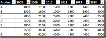
For my example, in order to be able to modify the table, I’m using a simple Excel table which looks like this:
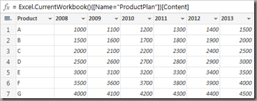
I’m using this table as the source for a new query in Power Query:
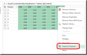
In order to transform the columns into rows, I select all columns with years and choose unpivot from the context menu:
Here is the result:
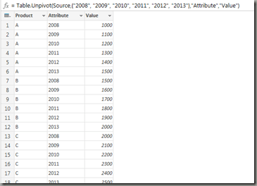
This was quite easy. For my example, I’m leaving the query like this (usually you would go ahead and rename the columns etc.).
Now, what happens if a new columns is added to my source table. Let’s assume we’re adding a year for 2014.
By clicking Refresh in the context menu of the Excel table resulting from my Power Query, the query is executed again. The result looks like this:
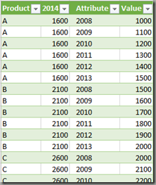
As you can see, the year 2014 is not included in the unpivot operation but became an additional column. This is clearly understandable if we look at the generated M script:
-
let
-
Source = Excel.CurrentWorkbook(){[Name=„ProductPlan“]}[Content],
-
Unpivot = Table.Unpivot(Source,{„2008“, „2009“, „2010“, „2011“, „2012“, „2013“},„Attribute“,„Value“)
-
in
-
Unpivot
Since the Table.Unpivot function names each column that is to be included in the unpivoted operation, the new column is not reflected by the query script.
In the analytical language R, this task would by easier, since the melt-function, which is the corresponding function for unpivoting data in R, takes the columns that are to be fixed when unpivoting. So assuming the table above has been loaded in R as a data frame df, the unpivot operation would look like
-
df_unpivot<-melt(df, id=c(„Product“))
But let’s get back to Power Query. In order to make our query aware of a different number of columns, we need to replace the constant column list with a variable one. Let’s do it step by step by modifying the script above.
First, we need a list of all the columns from our input table (Source):
-
let
-
Source = Excel.CurrentWorkbook(){[Name=„ProductPlan“]}[Content],
-
Unpivot = Table.Unpivot(Source,{„2008“, „2009“, „2010“, „2011“, „2012“, „2013“},„Attribute“,„Value“),
-
Cols = Table.ColumnNames(Source)
-
in
-
Cols
Modified code is shown in red. Please be aware of the comma at the end of the line starting with Unpivot=…
Also, quite interesting, we’re still having the Unpivot transformation from above in the M script, we’re just not showing it, as we use our recently created variable Cols as the output (in-clause). So the result is the list of column names from our table:
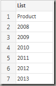
Usually, the first columns are to be fixed for the unpivot operation. So here, the function List.Skip is useful: We just skip the first column in order to get all the columns with the year values:
-
let
-
Source = Excel.CurrentWorkbook(){[Name=„ProductPlan“]}[Content],
-
Unpivot = Table.Unpivot(Source,{„2008“, „2009“, „2010“, „2011“, „2012“, „2013“},„Attribute“,„Value“),
-
Cols = Table.ColumnNames(Source),
-
ColsUnPivot=List.Skip(Cols, 1)
-
in
-
ColsUnPivot
Again, the modified part is shown in red (and again, take care of the comma). This gives us the desired list of columns:
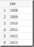
Now, all we have to do is to replace the constant list from the Unpivot function with the newly generated list ColsUnPivot. I’m moving the Unpivot operation to the end of the list and also use this as the query output. Here’s the resulting script:
-
let
-
Source = Excel.CurrentWorkbook(){[Name=„ProductPlan“]}[Content],
-
Cols = Table.ColumnNames(Source),
-
ColsUnPivot=List.Skip(Cols, 1),
-
Unpivot = Table.Unpivot(Source,ColsUnPivot,„Attribute“,„Value“)
-
in
-
Unpivot
Not surprisingly, the query returns exactly the same output as the query before. In order to see the difference, let’s add the year 2014 again to our source table and refresh the query from Power Query:
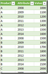
As you see, the result now contains the year 2014 on the rows, not on an extra column. This is exactly what we were trying to achieve.


Kommentare (0)