PDW v1/v2
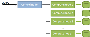
In my first post I wrote about the need of a consequently tuned and aligned database server system in order to handle a high data warehouse workload in an efficient way. A commonly chosen implementation for this is a massive parallel shared nothing architecture. In this architecture your data is distributed among several nodes, each with their own storage. A central node processes incoming queries, calculates the parallel query plan and sends the resulting queries to the compute nodes.In a simplified form, this architecture looks as shown below:
Since different vendors choose different detail strategies, from now on, I’m focusing on the Microsoft Parallel Data Warehouse, or in short, the Microsoft PDW. The PDW is Microsoft’s solution for MPP data warehouse systems. The PDW ships as an appliance, i.e. as a pre-configured system (hard- and software) of perfectly compatible and aligned components, currently available from HP and DELL.
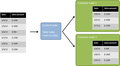
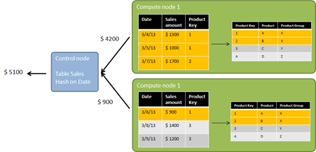
What happens if data is loaded into such a system? Let’s assume we have a table with 6 rows of sales and for simplicity, let’s assume we only have two compute nodes. In order to distribute the data among the compute nodes, a distribution keys needs to be chosen. This key will be used to determine the compute node for each row. Why don’t we just do a round robin distribution? I’m getting back to this point later in this post. The distribution key (table column) is used in a hash function to find a proper node. The hash function takes into account the data type of the distribution key, as well as the number of distributions. Actually, in PDW the table is also distributed on the compute node itself (8 different tables on different files/file groups) to get the optimal usage of the compute node’s cores and the optimal throughput to the underlying storage. For our example, let’s assume that the date values hash to the nodes as shown in this illustration:
As you see, each row of data is routed to a specific compute node (no redundancy). Doesn’t make this the compute node a single point of failure in the system? Actually no, because of the physical layout of the PDW. In PDW v2 two compute nodes share one JBOD storage system, one of them communicating actively with the JBOD, the other using the infiniband network connection. The compute nodes itself are “normal” SQL Server 2012 machines running on Hyper-V. If a compute node fails, the data is still reachable using the second compute node that is attached to this JBOD. The compute nodes form an active/passive cluster, therefore the spare node can take over, if a node fails. The damaged node may easily be repaired or replaced. A Hyper-V image for a compute node sits on the management node (which I omitted in the illustration above). And again, this is just a very broad overview of the architecture. You can find very detailed information on the technology here: http://www.microsoft.com/en-us/sqlserver/solutions-technologies/data-warehousing/pdw.aspx
With the example above, what happens if we query a single date? Since we distributed the table on the date, a single compute node contains the data for this query. The control node can pass the query to the nodes and has no more action to take. The compute node containing the data can directly stream the data to the client. The same would happen if we run a query that groups by Date (and potentially filters by some other columns). Now both compute nodes can separately compute the result and stream the result to the client. What you see from this example is
- In this case, two machines work in parallel and fully independently from each other
- Since we distributed on Date and the query uses Date in the grouping, no post processing is necessary (we call this an aggregation compatible query)
(if the distribution would have happened based on a round robin approach, there would never by an aggregation compatible query) - In order to get the best performance in this case, it’s important that the data is equally distributed between the compute nodes. In the worst case of all the data being queried sitting on only one of the compute nodes, this one node would have to do the full work. Choosing a proper distribution key can be challenging. I’m getting back to this in a subsequent post.
What happens if we run a query like the following?
-
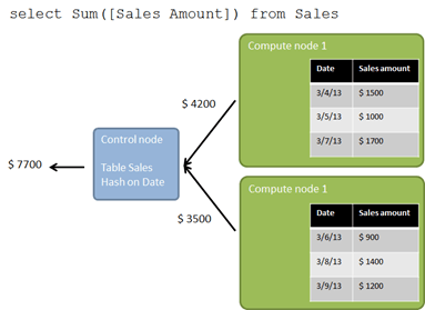
select Sum([Sales Amount]) from Sales
Again each compute node can compute the individual partial result but now these results need to be send to the control node to calculate the final result (so called partition move). However, in this example, the control node gets much less rows to process compared to the total amount of rows. Imagine millions or billions of rows being distributed to the compute nodes. The control node in this example would only get two rows with partial results (as we have two compute nodes in our example). So, this operation still fully benefits from the parallel architecture.
And this works for most kind of aggregations. For example, if you replace sum([Sales Amount]) with avg([Sales Amount]), the query optimizer would ask the compute nodes for the sum and count and compute the average in the final step.
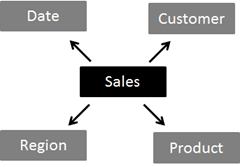
Ok, usually data models are more complicated (even in a data warehouse) than a single table. In a data warehouse we usually find a star (or snowflake) relationship between facts and dimensions. For the sales table above, this could look like this:
What happens now, if the query above is filtered by the product group, which is an attribute of the product dimension?
-
select sum([S.Sales Amount]) from Sales S
-
inner join Product P on S.ProductKey=P.ProductKey
-
where P.ProductGroup=‚X‘
How should we distribute the product table on the compute nodes in order to get good query performance? One option would be to distribute on the same key as the Sales. If we can do so, each compute node would see all products that are related to the sales that sit on this compute node and therefore answer the query without needing any data from other nodes (we would call this a distribution compatible query). However, the date is not a column in the product table (this wouldn’t make sense) so we cannot distribute the products in this way. It would work, if we had a SalesOrderHeader and SalesOrderDetail table, both joined and distributed on a SalesOrderID. But for the product dimension (as for most other dimensions too) we can go for a more straightforward approach. Fortunately, in a data warehouse, dimensions usually contain very few rows compared to the fact tables. It’s not uncommon to see over 98% of the data in fact tables. So for the PDW, it would make no difference if we put this table on all compute nodes. We call this a replicated table, while the Sales table itself is a distributed table. By making the Sales table distributed and the dimensions replicated, each compute node can answer queries that filter or group on dimension table attributes (columns) autonomically without needing data from other compute nodes.
Of course, this is just a very brief overview to show the basic concept. If we need to scale the machine, we could add more compute nodes and (after a redistribution of the data) can easily benefit from the higher computing power. This means we can start with a small machine and add more nodes as required which gives a great scalability. For the PDW v2 you can scale from about 50TB to about 6PB with a linear performance gain.
Also, PDW v2 offers a lot more features. Especially I’d like to mention the clustered column store index (CCI), which is a highly compressed, updatable in-memory storage of tabular data. Together with the parallel processing of the compute nodes this gives an awesome performance when querying data from the PDW. Also the seamless integration with Hadoop (via PolyBase) allows us to store unstructured data in a Hadoop file system and query both sources transparently from the PDW in the well known SQL syntax without IT needing to transfer the data into the relational database or to write map-reduce jobs.
Conclusion
Data Warehouses with large amount of data have challenges that go far beyond just storing the data. Being able to query and analyze the data with a good performance requires special considerations about the system architecture. When dealing with billions of rows, classical SMP machines can easily reach their limit. The MPP approach, that distributes data on multiple, independent compute nodes can provide a robust and scalable solution here. The Microsoft Parallel Data Warehouse is a good example for this approach that also includes features like in-memory processing (clustered column store index in v2) and a transparent layer on both structured and unstructured data (Hadoop).


Kommentare (0)