Custom Aggregates in DAX / BISM Tabular (part 2)

SQL Server Danali | PowerPivot 

This post combines two ideas

1. The calculation of a moving average (last 30 days) as shown in a previous post
2. Custom aggregations

What I want to show here today, is how we can influence the way our calculation works on higher levels. For this purpose I’m showing three different approaches:

1. The monthly (quarterly, yearly) total is defined as the last day’s moving average of the given date range.
   This corresponds to the original approach from my post about moving averages
2. The monthly (quarterly, yearly) total is defined as the average of all the moving averages on day level.
3. The monthly (quarterly, yearly) total is defined as the average of the sales amount of all days of that period (the moving average is only to be calculated on date level)

Of course, there are many more possibilities but I think the methods shown here, can be used for many other aggregation requirements.

Here are the three aggregations side by side.

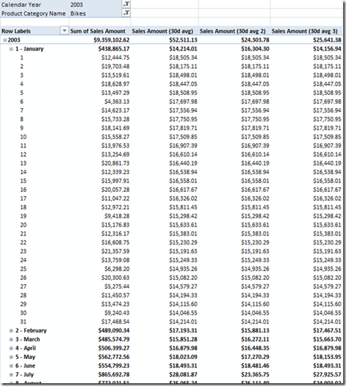
Although the values on higher levels of aggregation differ a lot, the daily values are identical (we just wanted to change the rollup method, not the calculation on a detail level).

Let’s start with the first one:

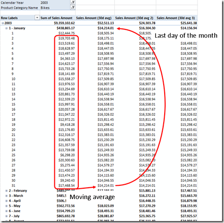
1. The monthly (quarterly, yearly) total is defined as the last day’s moving average of the given date range

This is shown here for our measure “Sales Amount(30 avg)”:

As shown in my previous post , the formula may look like this:

Since we use the expression LastDate(‘Date’[Date]) the last date of each period is used for the moving average – exactly what we wanted.

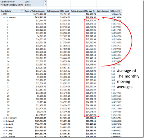
Average at month level as the average of the moving averages (day level)

In this approach, the monthly aggregate has to be calculated as the average of all the daily moving averages of that month. The picture shows what this means:

This might look pretty difficult. However, for our calculation we simply have to wrap the existing calculation in another Summarize – function.

This is the formula I used:

The blue part of the formula is exactly the same is in the first calculation. We’re just wrapping this in an additional Average function. Why does this still work on a day-level? Simply because the outer average computes the average of a single value in this case.

So, with just a minor change to the formula, we changed the method of aggregation quite a lot.

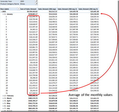
3. The monthly (quarterly, yearly) total is defined as the average of the sales amount of all days of that period

This sounds quite simple but in this case we have to distinguish two calculation paths:

• day level
• month level and above

The following picture shows the calculation for the monthly aggregate:

In order to split our computation paths we need to find out if we are on day level or not. Usually the IsFiltered(…) DAX function can be used for this purpose. However, since we have some columns with date granularity (date, day of month, day of year) in our date dimension, we would have to write something like IsFiltererd(‘Date’[Date]) || IsFiltered(‘Date’[Day of Month]) || …

To simplify this, I simple used a count of days in the following code. If we count only one day, we’re on day level. Of course, the count is the more expensive operation, but for this example, I leave it that way (the date table is not really big).

Again the blue part of the formula is exactly the same as in our first approach. This part is taken whenever we’re on a day level. On higher levels, the aggregate is computed as a simple (not moving) average of all daily values.

So, using the concepts of my previous post we were able to change the aggregation method to meet very sophisticated requirements.